Technical Support Document

A1.1 Introduction

Models are an important component of climate change impact projections. In general, quantitative evaluations of health impacts require projections of 1) physical climate changes, 2) future socioeconomic characteristics, and 3) the relationships between these factors and the health outcome of interest. Uncertainties exist in each of these areas, and aligning the spatial and temporal parameters used in climate models with epidemiological data to assess health outcomes can be challenging. Despite these challenges, health impact modeling continues to improve, increasing our understanding of the quantitative impacts associated with climate change (for example, Melillo et al. 2014; Tamerius et al. 2007; Post et al. 2012).^1,2,3

A1.2 Quantitative Evaluations of Health Impacts

Projecting Climate Change Impacts

Climate models are used to analyze past changes in the long-term averages and variations in temperature, precipitation, and other climate indicators and to make projections of how these trends may change in the future. Since there is no universally accepted set of metrics to identify the “best” climate models, it is standard practice to use an ensemble (a collection of simulations from different models) in order to present a range of results and provide a measure of the certainty in the results. In addition, because climate model results can depend on initial conditions (the state of the atmosphere and ocean at the moment the modeling run begins), even for a single model, multiple model simulations can be used to similarly present a range of results and improve understanding of variability. Climate model outputs may require additional processing, such as the use of downscaling methods when higher resolutions are needed, or coupling to an atmospheric chemistry model in order to examine and incorporate changes in local air quality.

Projections of climate changes are usually based on scenarios (or sets of assumptions) regarding how future emissions may change as a result of population, energy, technology, and economics. Over the past decade, climate change simulations were based primarily on emissions scenarios developed in the Intergovernmental Panel on Climate Change (IPCC) Special Report on Emissions Scenarios (SRES) .⁴ These scenarios were used as inputs to climate models in order to develop projections used in the Coupled Model Intercomparison Project Phase 3 (CMIP3). The global climate model (GCM) simulations included in CMIP use a standard experimental protocol so that their outputs can be compared. The IPCC Fifth Assessment Report⁵ drew upon model simulations from the Coupled Model Intercomparison Project Phase 5 (CMIP5), which collected simulation data from more recent models, used Representative Concentration Pathways (RCPs) in place of SRES scenarios, and incorporated updated historical forcing trends and other exogenous model inputs.

CMIP5 contains approximately 60 climate representations from 28 different modeling centers.⁶ The spatial resolution of most model grid cells is about 1° to 2° of latitude and longitude, or about 60 to 130 square miles. CMIP5 experiments simulate both

• the 20th century climate using the best available estimates of the temporal variations in external forcing factors (such as greenhouse gas concentrations, solar output, and volcanic aerosol concentrations); and
• the 21st century climate based on future greenhouse gas concentration pathways resulting from various emissions scenarios.

Four RCP emissions pathways were used for the CMIP5 simulations: RCP2.6, RCP4.5, RCP6.0, and RCP8.5. These pathways are named according to the increase in radiative forcing (a measure of the total change in Earth’s energy balance) projected for that pathway in the year 2100 relative to preindustrial levels, measured in Watts per square meter (Wm^-2). For example, RCP6.0 projects that the end-of-century radiative forcing increase will be 6.0 Wm^-2 above preindustrial levels. The range of simulated global average surface temperature changes under both SRES and RCPs is shown in Figure A1.1.

 

Figure A1.1: Scenarios of Future Temperature Rise

Projected global average temperature rise for specific emissions pathways (left) and concentration pathways (right) relative to the 1901_1960 average. Shading indicates the range (5thto 95th percentile) of results from a suite of climate models. Projections in 2099 are indicated by the bars to the right of each panel. In all cases, temperatures are expected to rise, although the difference between lower and higher pathways is substantial.

The left panel shows the two main CMIP3 scenarios (SRES) used in this assessment: A2 assumes continued increases in emissions throughout this century, and B1 assumes significant emissions reductions beginning around 2050. The right panel shows the newer CMIP5 scenarios using Representative Concentration Pathways (RCPs) . CMIP5 includes both lower and higher pathways than CMIP3. The lowest concentration pathway shown here, RCP2.6, assumes immediate and rapid reductions in emissions and would result in about 2.5°F of warming in this century. The highest pathway, RCP8.5, roughly similar to a continuation of the current path of global emissions increases, is projected to lead to more than 8°F warming by 2100, with a high-end possibility of more than 11°F. (Data from CMIP3, CMIP5, and NOAA NCEI). (Figure source: adapted from Melillo et al. 2014)¹

Projecting Socioeconomic Development

Along with the RCPs, used to provide a range of possible future greenhouse gas concentrations for climate models, the modeling of climate change impacts can be improved by acknowledging scenarios that describe future societal characteristics. For the IPCC’s Fifth Assessment Report,⁵ impact modelers discussed the use of new scenarios constructed from three building blocks:

• Representative Concentration Pathways (RCPs)
• Shared Socioeconomic Pathways (SSPs)
• Shared Climate Policy Assumptions (SPAs)

Shared Socioeconomic Pathways define plausible alternative states of global human and natural societies at a macro scale, including qualitative and quantitative factors such as demographic, political, social, cultural, institutional, lifestyle, economic, and technological variables and trends. Also included are the human impacts on ecosystems and ecosystem services, such as air and water quality.^7,8,9

As with the IPCC Fifth Assessment Report, SSPs are not explicitly used in the analyses highlighted in this assessment. However, because these scenarios are likely to be used by the impacts modeling community over the next few years, placing the approach taken in this assessment in context is a valuable exercise.

Five reference SSPs, referred to as SSP1 through SSP5,⁹ describe challenges to adaptation (efforts to adapt to climate change) and mitigation (efforts to reduce the amount of climate change) that change over time irrespective of climate change.^7,8,9 Although the SSPs describe broad-scale global trends across multiple sectors, these trends are relevant to projections of health impacts in the United States; trends within each SSP represent different challenges for maintaining and improving the health of Americans. For example, future vulnerability to changing concentrations of air pollutants, particularly ozone, will in part depend on demographics, urbanization, policies to control air pollutants, and hemispheric transport of emissions from areas outside the region.

The combination of RCP6.0 (used by most of the analyses highlighted in the Temperature-Related Death and Illness, Air Quality Impacts, Vector-Borne Diseases, and Water-Related Illness chapters—see Section A1.2) and the population parameters for the SRES B2 emissions pathway (used in the extreme heat and ozone analyses highlighted in Ch. 2: Temperature-Related Death and Illness and Ch. 3: Air Quality Impacts) can be partially mapped to the SSP2 storyline.^9,10 SSP2 depicts a world where global health improves at an intermediate pace. Under SSP2, multiple factors contribute to some countries making slower progress in reducing health burdens, including, in some low-income countries, high burdens of climate-related diseases combined with moderate to high population growth. In the United States, challenges to public health infrastructure and health care under this socioeconomic pathway could include inadequate resources and international commitment for 1) integrated monitoring and surveillance systems, 2) research on and modeling of the health risks of climate change, 3) iterative management approaches, 4) training and education of health care and public health professionals and practitioners, and 5) technology development and deployment.⁷

The SSPs do not include any explicit climate policy assumptions. This role is reserved for the Shared Climate Policy Assumptions (SPAs) which capture key policy attributes such as the goals, instruments, and obstacles of mitigation and adaptation measures up to the global and century scale.¹¹ In this way, the SPAs provide the link between RCPs and SSPs by allowing for a variety of alternative socioeconomic evolutionary paths to be coupled with a library of climate model simulations created using the RCPs. SPAs are also not used in the analyses highlighted in this assessment.

Projecting Health Outcomes

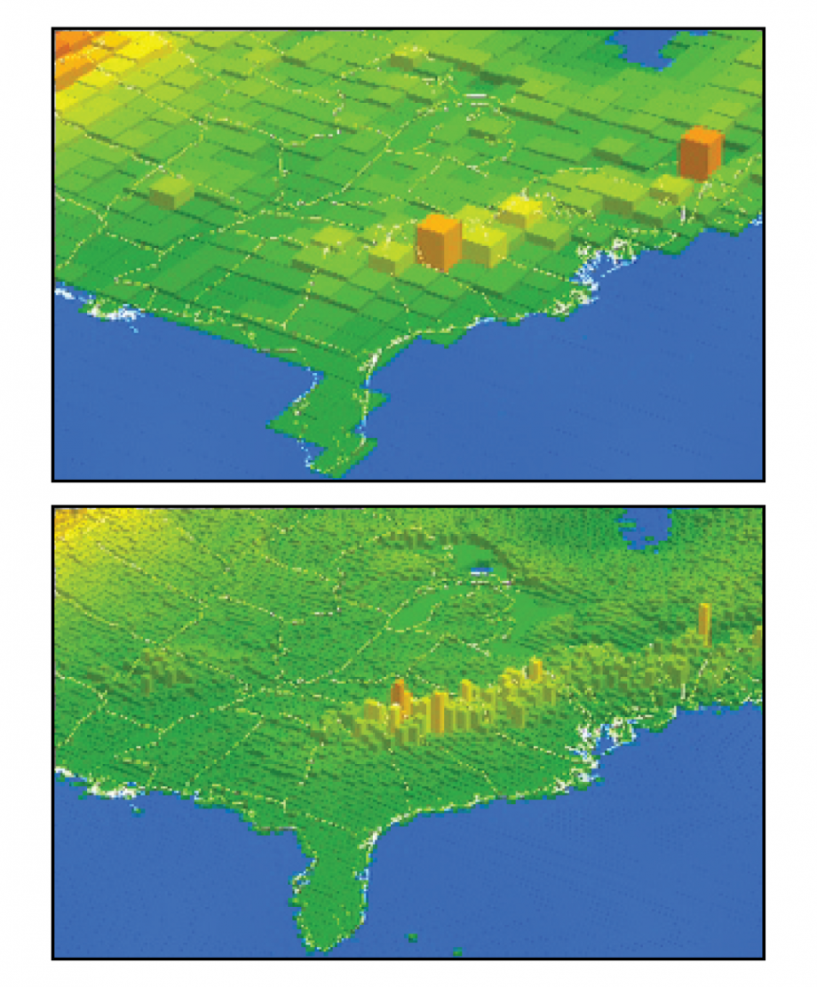
Public health officials often require information on health risks at relatively local geographic scales. Climate models, on the other hand, are better at projecting changes on national to global scales and over timescales of decades to centuries. Figure A2.2 shows two illustrative resolutions for eastern North American topography. The top figure has a grid cell resolution of 68 miles by 68 miles, which is comparable to high resolution global models with projections at a 1° latitude by 1° longitude resolution. The lower figure shows how the same topography would look using smaller grid cells with a resolution of 19 miles by 19 miles. The finer detail at the higher resolution (note, for example, the better representation of the elevation changes of the Appalachian Mountains) would potentially improve a model’s ability to provide local information, as temperature, winds, and other features of the model simulation are all influenced by topography. On the other hand, models with higher resolution are not necessarily better at capturing large-scale climate changes and weather patterns.

In addition to higher spatial resolutions, public health officials are also generally most interested in short-term projections of future conditions (for example, one to five years). This is in part due to the fact that these officials work in resource-constrained environments where relative priorities and associated funding decisions can shift, often quickly. In addition, they provide services to populations with characteristics that are likely to change in response to changing economic conditions, immigration patterns, or impacts of extreme weather events. In this short timeframe, public health officials typically focus on information regarding the timing and magnitude of specific events or combinations of events that would stress existing programs and systems (for example, heat waves, tropical storms, wildfires, and air quality events). The one- to five-year information requirements of public health providers can contrast with the information climate modelers can develop, which project future conditions for timescales of decades to centuries and often derive impacts in 2050 or 2100. Climate models provide less guidance in terms of changes in near-term impacts because short-term variability from natural sources such as ocean circulation can obscure the long-term climate trends produced by increasing greenhouse gas concentrations. As such, climate projections over longer time periods typically serve more as a guide to emerging issues and as an input to longer-range planning.

A1.3 Modeling Highlighted in the Assessment

The four chapters that highlight modeling studies conducted for this assessment (Temperature-Related Death and Illness, Air Quality Impacts, Vector-Borne Diseases, and Water-Related Illness) analyzed a subset of the full CMIP5 dataset (see Table A1.1). The air quality analyses required the most intensive processing of the CMIP5 model output; calculating air quality changes at the appropriate geographic scale requires modelers to use a technique known as dynamical downscaling to generate climate data at the desired small-scale resolution, and then run an atmospheric chemistry model, both of which are computationally intensive processes. Thus the ozone analysis was limited to two model–scenario examples (see Table A1.1). By contrast, the water-related illness analyses examined results from 21 of the CMIP5 models, though only for one particular scenario .

In general, the authors of the studies highlighted in this assessment used historical data in order to calibrate their historical results and to improve geographic resolution. These downscaling approaches determine the climate signal by taking the difference between the modeled future and the modeled historical period at the grid cell resolution (often averaged over 30 years). This climate signal can then be added to observed historical data at a resolution potentially much finer than the model grid cell scale. For example, any given weather station might be, on average, cooler in the summer than the grid cell average because it is located next to a lake. By adding the modeled climate signal to the historical data from the weather station, the projected future temperatures can more effectively account for microclimate effects, from lakes or hills for example, that are consistent with historical variation at a spatial resolution smaller than the modeled grid scale. More sophisticated calibrations can also adjust model variability to match historical variability by using a technique known as quantile mapping.¹²

The modeling studies highlighted in this assessment use several approaches. The three different historical reference periods used in the highlighted studies (1985–2000, 1992–2007, and 1976–2006) are slightly warmer than the 1971–2000 period used in the 2014 National Climate Assessment (NCA), by 0.3°F to 0.8°F. In addition, different sets of climate models were used.

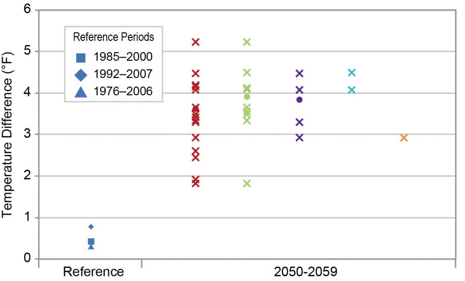
A sensitivity analysis was conducted to test for two potential impacts of using different modeling approaches: the use of different historical reference periods and the use of different sets of CMIP5 models. Figure A1.3 shows the change in temperature from the 2014 NCA reference period (1971–2000) for three historical reference periods used in the studies highlighted (first column). The differences among these three historical reference periods are small compared with the warming projected for the middle of this century by the different sets of models used (second column). For the sets of 21, 11, and 5 models used in the studies of Vibrio/Alexandrium species, Gambierdiscus species, and Lyme disease, respectively, the multi-model mean warming for the middle of the 21st century are within 0.5°F of each other, although the set of 11 models does not include a few of the cooler models and the set of 5 models spans a narrower range. The two models used in the extreme temperature study are slightly warmer than the mean of the entire set of models, while the single model used in the air quality (ozone) study is slightly cooler. However, these differences in mean warming among the five approaches shown in the second column are small compared to projected warming.

Each modeling approach requires different input from the climate models. For example, the temperature mortality analysis required only temperature data, while the analysis in the Water-Related Illness chapter used sea surface temperature data. However, the ambient air quality modeling required temperature, precipitation, ventilation, and other data in order to provide boundary conditions for the dynamical downscaling approach. Besides climate data, modeling teams also used other inputs. The main sources of additional data were the Integrated Climate and Land Use Scenarios (ICLUS) model for population projections and the Environmental Benefits Mapping and Analysis Program (BenMAP) model for baseline mortality data, which were used for the extreme temperature and air quality modeling efforts.^13,14 The analysis in the Water-Related Illness chapter required salinity, light, and other oceanographic data not provided by the CMIP5 models.

The modeling approaches also included different geographic scales. The Water-Related Illness analyses examined individual bodies of water such as the Chesapeake Bay, Puget Sound, and the Gulf of Mexico. The vector-borne disease projections of Lyme disease concentrated on the 12 U.S. states where Lyme disease is most prevalent. The temperature mortality analysis examined 209 U.S. cities that had sufficient data for a historical epidemiology analysis. The ozone analysis was able to address the entire contiguous United States.         

A1.4 Sources of Uncertainty

The use of the term “uncertainty” in climate assessments refers to a range of possible futures. Uncertainty about the future climate arises from the complexity of the climate system and the ability of models to represent timing, magnitude, and location of changes, as well as the difficulties in predicting the decisions that society will make. There is also uncertainty about how climate change, in combination with other stressors, will affect people and natural systems.¹

 

Figure A1.4: Sources of Uncertainty

Examples of sources of uncertainty in projecting impacts of climate change on human health . The left column illustrates the exposure pathway through which climate change can affect human health. The right column lists examples of key sources of uncertainty surrounding effects of climate change at each stage along the exposure pathway.

Though quantitative evaluations of climate change impacts on human health are continually improving, there is always some degree of uncertainty when using models to gain insight into future conditions (see Figure A1.4). The presence of uncertainty, or the fact that there is a range in potential outcomes, does not negate the knowledge we have, nor does it mean that actions cannot be taken. Everyone makes decisions, in all aspects of their life, based on limited knowledge or certainty about the future. Decisions like where to go to college or what job to take, what neighborhood to live in or which restaurant to eat in, whom to befriend or marry, and so on are all made in light of uncertainty, which can sometimes be considerable. Recent years have seen considerable progress in the development of improved methods to describe and deal with uncertainty in modeling climate change impacts on human health (for example, Melillo et al. 2014; Tamerius et al. 2007; Post et al. 2012).^1,2,3

Uncertainty in Projecting Climate Change

Two of the key uncertainties in projecting future global temperatures are 1) uncertainty about future concentrations of greenhouse gases, and 2) uncertainty about how much warming will occur for a given increase in greenhouse gas concentrations. Future concentrations depend on both future emissions and how long these emissions remain in the atmosphere (which can vary depending on how natural systems process those emissions). Because of uncertainty in future greenhouse gas concentrations, climate modelers analyze multiple future emissions pathways in order to determine the range of varying impacts of lower emissions compared to higher emissions. In terms of how much warming will occur for a given increase in greenhouse gas concentrations, the most recent assessment by the IPCC found the most likely response of the climate system to a doubling of carbon dioxide (CO₂) concentrations, referred to as the sensitivity in climate models, lies between a 1.5°C and 4.5°C (2.7°F to 8.1°F) increase in global average temperature (see Figure A1.1).⁵

Climate scientists have greater confidence in predicting the average temperature of the whole planet than what the temperature will be in any given region or locale. Global average temperatures may not, however, be particularly informative for determining health impacts at a local scale. An increase in global temperatures will, at local scales, result in different warming rates in different locations, different seasonal warming rates, different warming rates during the day compared to the night, and different changes in day-to-day or year-to-year variability. Despite these possible differences, it is highly likely that warming will occur almost everywhere.²¹ In addition to temperature, changes in precipitation, humidity, and weather systems are all important drivers of local impacts. However, future changes in these variables are less certain than changes in temperature.

Uncertainty in Public Health Surveillance and Monitoring

Improvements in understanding future health impacts can result from better understanding current health impacts. Obtaining this understanding is complicated by the fact that, in the United States, there is no single source of health data and surveillance often involves acquiring, analyzing, and interpreting data from several sources collected using potentially different techniques and systems.^22,23 This is further complicated by a number of additional limitations, including the fact that data are often incomplete, may not include a representative sample of all members of society, and rely on reporting of disease status. Estimates of disease patterns or trends may also vary across geographic locations.²³ Understanding the surveillance and monitoring limitations regarding population health data and spatial variability can enable more accurate estimations of the confidence in the links between health impacts and climate drivers, and this can be used to estimate uncertainty in future projections of health impacts.

Having complete socioeconomic, geographic, demographic, and health data at an individual level for everyone would improve our understanding of connections between these attributes and deaths and illnesses. However, such complete data are not available for both practical and confidentiality reasons. Mandatory reporting, disease records, and administrative sources, including data from medical records or vital records, can be used to estimate counts of given health impacts and these counts can be divided by population estimates to produce health impact rates. Uncertainty in the data can differ depending on the type of population health estimate and the existing surveillance data source used (such as using registries versus surveys).

In addition to uncertainty regarding the quality and usefulness of data, confidence in estimates of health impacts depends on the extent of useable data. In general, the larger the data set (larger populations or longer time periods), and the more common the health condition, the more confidence there is in estimated rates, and changes in those rates, across time periods, demographic groups, or other attributes.²²

Uncertainty in Estimating Stressor -Response Relationships

Exposure–response or stressor–response relationships describe the change in the health status associated with different levels of exposure to a stressor or concentration of a stressor (also see Ch. 1: Introduction, Section 1.4). Some environmental exposures, such as air quality and ambient temperature, have a relatively direct effect on deaths and illness, which is captured in stressor-response relationships in epidemiological studies. For example, increases in temperature can affect a range of chronic illnesses and infectious diseases. In other situations, climate change will have health effects through intermediaries such as changes in ecological conditions like pollen distribution (causing allergies) and the distribution of infectious disease pathogens and vectors (causing vector-borne, foodborne, and waterborne infectious diseases). Modeling exposure–response relationships can be particularly challenging for outcomes involving multiple intermediary stressors along an exposure pathway, each of which may be influenced by climate change. Even for relatively direct impacts, the same exposure can produce different responses for different health outcomes. Moreover, responses for a given exposure can vary by location (for example, different impacts of extreme heat in dry areas versus humid areas) and across sub-populations (different socioeconomic and demographic groups). For each pairing of exposure and health response, the exposure–response relationship may be represented as a quantitative estimate (such as the increase in number of deaths for a 1°F increase in maximum temperature) or in a qualitative manner (such as a determination that increases in extreme precipitation events may increase exposure to indoor molds).

In recent decades, progress has been made in modeling exposure–response relationships for a wide range of climate-sensitive environmental exposures and health responses. For example, we have gained a better understanding in recent years of the relationships between exposure to varying temperatures, concentrations of ozone and fine particulate matter, and the health response in terms of a range of illnesses and premature death (for example, Samoili et al. 2005. Bobb et al. 2014; see also Ch. 2: Temperature-Related Death and Illness and Ch. 3: Air Quality Impacts).^24,25 Quantitative exposure–response functions are often used in understanding how health risks from these exposures vary across locations; these are also used in modeling efforts to project the health impacts of climate change in specific locations. However, it is important to carefully consider uncertainty when developing and using exposure–response functions, as the environmental processes affecting human health are complex.

Exposure–response functions may not remain constant over time or space. One source of uncertainty arises from the potential that high levels of exposure could be associated with proportionately larger effects compared to low levels of exposure (non-linearity, see for example Gasparrini 2014 and Burnett et al 2014).^26,27 Further, as the nature of the exposure and the potential for changes in human behavior and adaptive capacity change over time, so can the response function change. Representing health response for a singular point estimate of exposure instead of a range of exposure values could lead to imprecise assessment of the health risk. The large amounts of data required for reliable and accurate estimation of exposure–response functions may not be available at suitable resolutions for all locations (for example, Hubbell et al 2009).²⁸ In some cases, estimating health outcomes by using exposure–response functions from other locations in the absence of reliable locally specific exposure–response relationships introduces uncertainty (for example, Wardekker et al. 2012).²⁹ The exposure_–response estimates may also vary within sub-populations in a location, being relatively high for particularly vulnerable communities (for example, the elderly population will have a higher exposure–response relationship from extreme heat compared to the rest of the population).

Another challenge in characterizing the relationship between exposure and health impacts is determining when a relationship is correlative, as opposed to causative. For example, statistical analyses would adjust for other factors that could be influencing health outcomes, such as age, race, year, day of the week, insurance status, and the concentrations of other air pollutants. Evaluating and integrating evidence across epidemiological, toxicological, and controlled human exposure studies allows researchers to conclude whether there is a causal relationship between human exposure to air pollution and a given health outcome. As evidence mounts, as is the case for associations between ozone concentration and adverse health impacts,^{30,31,32,33,34,35} the hypothesis of a causal relationship is strengthened, and observed exposure–response associations can be used with greater confidence.

Users of exposure–response relationships in risk assessments or disease burden projection need to carefully consider the context in which the estimates were derived prior to their use. Carefully designed meta-analyses, leveraging the information obtained from multiple studies, can provide summary estimates of relationships and ensure consistency in application (for example, Normand 1999).³⁶

Approach to Reporting Uncertainty in Key Findings

Despite the sources of uncertainty described above, the current state of the science allows an examination of the likely direction of and trends in the health impacts of climate change. Over the past ten years, the models used for climate and health assessments have become more useful and more accurate (for example, Melillo et al. 2014; Tamerius et al. 2007; Post et al. 2012).^1,2,3 This assessment builds on that improved capability. A more detailed discussion of the approaches to addressing uncertainty from the various sources can be found in the Guide to the Report (Front Matter) and Appendix 4: Documenting Uncertainty: Confidence and Likelihood.

Two kinds of language are used when describing the uncertainty associated with specific statements in this report: confidence language and likelihood language. Confidence in the validity of a finding is based on the type, amount, quality, strength, and consistency of evidence and the degree of expert agreement on the finding. Confidence is expressed qualitatively and ranges from low confidence (inconclusive evidence or disagreement among experts) to very high confidence (strong evidence and high consensus).

Likelihood language describes the likelihood of occurrence based on measures of uncertainty expressed probabilistically (in other words, based on statistical analysis of observations or model results or on expert judgment). Likelihood, or the probability of an impact, is a term that allows a quantitative estimate of uncertainty to be associated with projections. Thus likelihood statements have a specific probability associated with them, ranging from very unlikely (less than or equal to a 1 in 10 chance of the outcome occurring) to very likely (greater than or equal to a 9 in 10 chance). The likelihood rating does not consider severity of the health risk or outcome, particularly as it relates to health risk factors not associated with climate change, unless otherwise stated in the Key Finding.

Each Key Finding includes confidence levels; where possible, separate confidence levels are reported for 1) the impact of climate change, 2) the resulting change in exposure or risk, and 3) the resulting change in health outcomes. Where projections can be quantified, both a confidence and likelihood level are reported. Determination of confidence and likelihood language involves the expert assessment and consensus of the chapter author teams. The author teams determine the appropriate level of confidence or likelihood by assessing the available literature, determining the quality and quantity of available evidence, and evaluating the level of agreement across different studies. Often, the underlying studies will provide their own estimates of uncertainty and confidence intervals. When available, these confidence intervals are used by the chapter authors in making their own expert judgments.

This assessment relies on two metrics to communicate the degree of certainty in Key Findings. See Appendix 4: Documenting Uncertainty for more on assessments of likelihood and confidence.

References

- , 2004: Ozone and short-term mortality in 95 US urban communities, 1987-2000. JAMA: The Journal of the American Medical Association, 292, 2372-2378. doi:10.1001/jama.292.19.2372 | Detail
- , 2014: Heat-related mortality and adaptation to heat in the United States. Environmental Health Perspectives, 122, 811-816. doi:10.1289/ehp.1307392 | Detail
- , 2014: An integrated risk function for estimating the global burden of disease attributable to ambient fine particulate matter exposure. Environmental Health Perspectives, 122, 397-403. doi:10.1289/ehp.1307049 | Detail
- , 2014: Health in the new scenarios for climate change research. International Journal of Environmental Research and Public Health, 11, 30-46. doi:10.3390/ijerph110100030 | Detail
- 2009: Land-Use Scenarios: National-Scale Housing-Density Scenarios Consistent with Climate Change Storylines (Final Report). EPA/600/R-08/076F. 137 pp., Global Change Research Program, National Center for Environmental Assessment, U.S. Environmental Protection Agency, Washington D.C. URL | Detail
- 2013: Integrated Science Assessment for Ozone and Related Photochemical Oxidants. Array, 1251 pp., U.S. Environmental Protection Agency, National Center for Environmental Assessment, Office of Research and Development, Research Triangle Park, NC. URL | Detail
- cited 2014: Environmental Benefits Mapping and Analysis Program--Community Edition (BenMAP-CE). U.S. Environmental Protection Agency. URL | Detail
- , 2012: Estimating the national public health burden associated with exposure to ambient PM2.5 and ozone. Risk Analysis, 32, 81-95. doi:10.1111/j.1539-6924.2011.01630.x | Detail
- , 2015: The geographic distribution and economic value of climate change-related ozone health impacts in the United States in 2030. Journal of the Air & Waste Management Association, 65, 570-580. doi:10.1080/10962247.2014.996270 | Detail
- , 2014: Modeling exposure-lag-response associations with distributed lag non-linear models. Statistics in Medicine, 33, 881-899. doi:10.1002/sim.5963 | Detail
- , 2009: Methodological considerations in developing local-scale health impact assessments: Balancing national, regional, and local data. Air Quality, Atmosphere & Health, 2, 99-110. doi:10.1007/s11869-009-0037-z | Detail
- , 2015: Effects of climate change on residential infiltration and air pollution exposure. Journal of Exposure Science and Environmental Epidemiology, Published online 27 May 2015. doi:10.1038/jes.2015.38 | Detail
- 2000: Special Report on Emissions Scenarios. A Special Report of Working Group III of the Intergovernmental Panel on Climate Change. Cambridge University Press, 570 pp. URL | Detail
- 2013: Climate Change 2013: The Physical Science Basis. Contribution of Working Group I to the Fifth Assessment Report of the Intergovernmental Panel on Climate Change. 1535 pp., Cambridge University Press, Cambridge, UK and New York, NY. doi:10.1017/CBO9781107415324 | Detail
- , 2015: A framework for examining climate-driven changes to the seasonality and geographical range of coastal pathogens and harmful algae. Climate Risk Management, 8, 16-27. doi:10.1016/j.crm.2015.03.002 | Detail
- , 2009: Long-term ozone exposure and mortality. New England Journal of Medicine, 360, 1085-1095. doi:10.1056/NEJMoa0803894 | Detail
- , 2011: Meta-analysis of the association between short-term exposure to ambient ozone and respiratory hospital admissions. Environmental Research Letters, 6, 024006. doi:10.1088/1748-9326/6/2/024006 | Detail
- , 2015: Effects of ocean warming on growth and distribution of dinoflagellates associated with ciguatera fish poisoning in the Caribbean. Ecological Modelling, 316, 194-210. doi:10.1016/j.ecolmodel.2015.08.020 | Detail
- , 2002: Healthy People 2010 Criteria for Data Suppression. 12 pp., National Center for Health Statistics, Hyattsville, MD. URL | Detail
- , 2014: A new scenario framework for climate change research: The concept of shared climate policy assumptions. Climatic Change, 122, 401-414. doi:10.1007/s10584-013-0971-5 | Detail
- , 2009: Decadal Prediction. Bulletin of the American Meteorological Society, 90, 1467-1485. doi:10.1175/2009bams2778.1 | Detail
- , 2014: Climate Change Impacts in the United States: The Third National Climate Assessment. U.S. Global Change Research Program, 841 pp. doi:10.7930/J0Z31WJ2 | Detail
- , 2015: Climate change influences on the annual onset of Lyme disease in the United States. Ticks and Tick-Borne Diseases, 6, 615-622. doi:10.1016/j.ttbdis.2015.05.005 | Detail
- 2015: Health, United States, 2014: With Special Feature on Adults Aged 55-64. 473 pp., National Center for Health Statistics, Centers for Disease Control and Prevention, Hyattsville, MD. URL | Detail
- , 1999: Meta-analysis: Formulating, evaluating, combining, and reporting. Statistics in Medicine, 18, 321-359. doi:10.1002/(SICI)1097-0258(19990215)18:3<321::AID-SIM28>3.0 | Detail
- , 2014: A new scenario framework for climate change research: The concept of shared socioeconomic pathways. Climatic Change, 122, 387-400. doi:10.1007/s10584-013-0905-2 | Detail
- , 2015: The roads ahead: Narratives for shared socioeconomic pathways describing world futures in the 21st century. Global Environmental Change, In press. doi:10.1016/j.gloenvcha.2015.01.004 | Detail
- , 2012: Variation in estimated ozone-related health impacts of climate change due to modeling choices and assumptions. Environmental Health Perspectives, 120, 1559-1564. doi:10.1289/ehp.1104271 | Detail
- , 2005: Estimating the exposure-response relationships betwen particulate matter and mortality within the APHEA multicity project. Environmental Health Perspectives, 113, 88-95. doi:10.1289/ehp.7387 | Detail
- , 2015: Projections of temperature-attributable premature deaths in 209 U.S. cities using a cluster-based Poisson approach. Environmental Health, 14. doi:10.1186/s12940-015-0071-2 | Detail
- , 2007: Climate and human health: Synthesizing environmental complexity and uncertainty. Stochastic Environmental Research and Risk Assessment, 21, 601-613. doi:10.1007/s00477-007-0142-1 | Detail
- , 2014: A new scenario framework for climate change research: Scenario matrix architecture. Climatic Change, 122, 373-386. doi:10.1007/s10584-013-0906-1 | Detail
- , 2014: Evaluating potential response-modifying factors for associations between ozone and health outcomes: A weight-of-evidence approach. Environmental Health Perspectives, 122, 1166-1176. doi:10.1289/ehp.1307541 | Detail
- , 2014: Ch. 2: Our Changing Climate. Climate Change Impacts in the United States: The Third National Climate Assessment, , U.S. Global Change Research Program, 19-67. doi:10.7930/J0KW5CXT | Detail
- , 2012: Health risks of climate change: An assessment of uncertainties and its implications for adaptation policies. Environmental Health, 11, Article 67. doi:10.1186/1476-069x-11-67 | Detail
- , 2004: Hydrologic implications of dynamical and statistical approaches to downscaling climate model outputs. Climatic Change, 62, 189-216. doi:10.1023/B:CLIM.0000013685.99609.9e | Detail